Solar bursts may be much stronger than your highest available noise calibrator level. The following discussion suggests a way that you may be able to estimate the level of these bursts from your Radio-SkyPipe chart using your present calibrator. The method could also be used to estimate signal levels that fall between your calibration levels. We assume that you are using a receiver with NO AGC, such as a Jove Receiver and that you are feeding a standard sound card with a audio signal level that does not approach the maximum input level capabilities of the card.
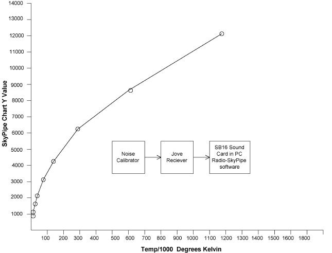
Using a homebrew noise generator (calibrated against an RF2010 noise generator), a Jove Receiver, and a PC using an old SoundBlaster 16 sound card, and Radio-SkyPipe software, I produced a table of SkyPipe Y chart values vs. input noise temperature levels (in 1000s of degrees Kelvin)
| Temp / 1000 Deg. K | Average Y Level |
| 4.8 | 918 |
| 9.3 | 1175 |
| 18 | 1640 |
| 36 | 2208 |
| 72 | 3161 |
| 143 | 4351 |
| 286 | 6278 |
| 569 | 8599 |
| 1136 | 12307 |
How did I get the average Y values? After all, those signals look very "grassy" on the chart and it is hard to estimate exactly what the average level is on an area of the chart just by looking at it. SkyPipe has a feature that you may not have used but is very handy for this type of thing. Simply use the zoom feature so that the area you want to measure covers the the visible area of the chart. Then right click on the chart and select "Get Avg for View". The average Y value for the visible portion of the chart will appear in the status bar.
Now that I had the table I was able to produce a graph:
The shape of the graph looked very much like a square function so I decided to try plotting the same data this time using the the square root of the Temp/1000 degrees Kelvin for the X axis. The result was very encouraging:
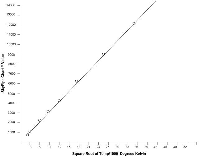
Plotting the data in this manner produced a very good approximation of a straight line. With this and some simple algebra it became evident that one could make good estimates of levels for which no calibration point was available. You could just look at the graph and estimate the level. Pick the level shown on the chart for which you are interested. For example, the part of the chart you were interested in had an average value of 11000. The corresponding value of the X axis would be roughly around 34. Square this value and you get 1156. The temperature corresponding to a Y value of 11000 is thus roughly 1,200,000 degrees Kelvin (You didn't forget that our chart was in 1000's of degrees did you?)
Another approach to estimating uses the slope of this graph's line. (There are probably better ways to do this but I prefer to keep the math simply stepped.) The slope of a straight line is the RISE / RUN , that is, the change in Y axis per change in X axis. We can find the slope using two points on our line. Arbitrarily, I will choose the point for Y=4351 and the point where Y=12307. These points are far enough apart that error should be small.
slope = (Y2 - Y1) / (X2 - X1) hint: use the larger coordinate pair for X2 and Y2
slope = (12307 - 4351) / (33.7 - 11.96) = 7956/21.74 = 367
Now that we have the slope we find an unknown coordinate for any other point on the line by comparing it with a known point's coordinates. To do this we use the same formula for slope. In this case, we want to find an unknown X value that pairs with a particular Y value that we can read off the strip chart. For example, our strip chart shows a solar burst that extends all the way up to a Y value of 18000. Our highest calibration level only went up to 12307 on the strip chart. What would the equivalent temperature of this burst be?
slope = (Y2 - Y1) / (X2 - X1) [measured above to be 367]
367 = (18000 - 12307) / (X2 - 33.7) = 5693 / (X2 - 33.7)
rearrange a little to get X2 on the left:
X2 = (5693 /367) + 33.7
X2 = 15.5 + 33.7 = 49.2
49.2 is the square root of our desired value so we must square it.
49.2^2 = 2420.6 and then we multiply by 1000 to put it into degrees
2,420,600 degrees K is our answer. Of course, this level of accuracy is unjustified so we would probably just say that the burst was about 2.4 million degrees.
This seems to work well with the experimental setup that I used, but different receivers and sound cards may produce different results. The slope defined here is not universal. You will have to redefine the slope of the for your system every time you make adjustments in the receiver volume, computer mixer settings, etc. If you cannot achieve a straight line for the square root of the temp vs the chart value you may be driving your sound card too hard, the sound card may have a different level conversion characteristic, or your receiver may be compressing under the strong signal levels.
For a good example of equations applied to convert to degrees Kelvin equivalent antenna temperature see Jim Brown's example at the NJ3BRO observatory.
Help Index | Radio-Sky Publishing Home